Wind energy has become one of the cornerstones of modern energy systems. It is renewable, scalable, and plays a critical role in reducing greenhouse gas emissions and dependence on fossil fuels. For many regions, wind farms are no longer an exception but a standard part of energy infrastructure planning.

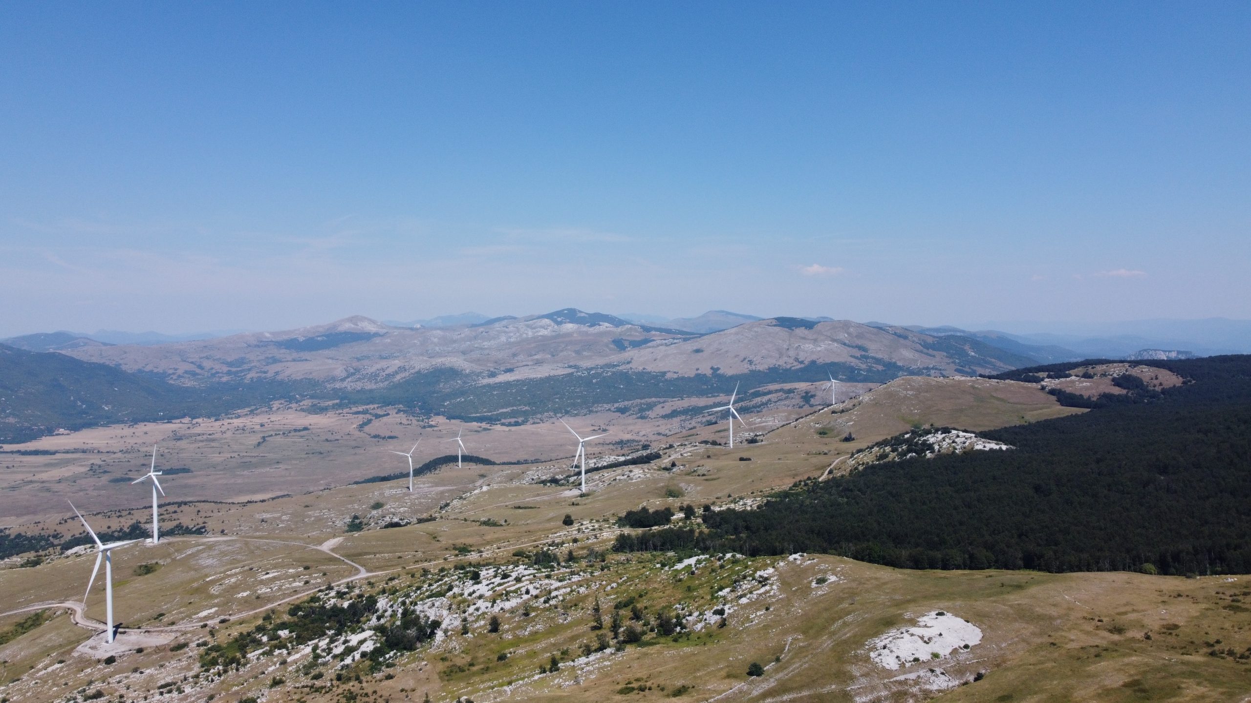
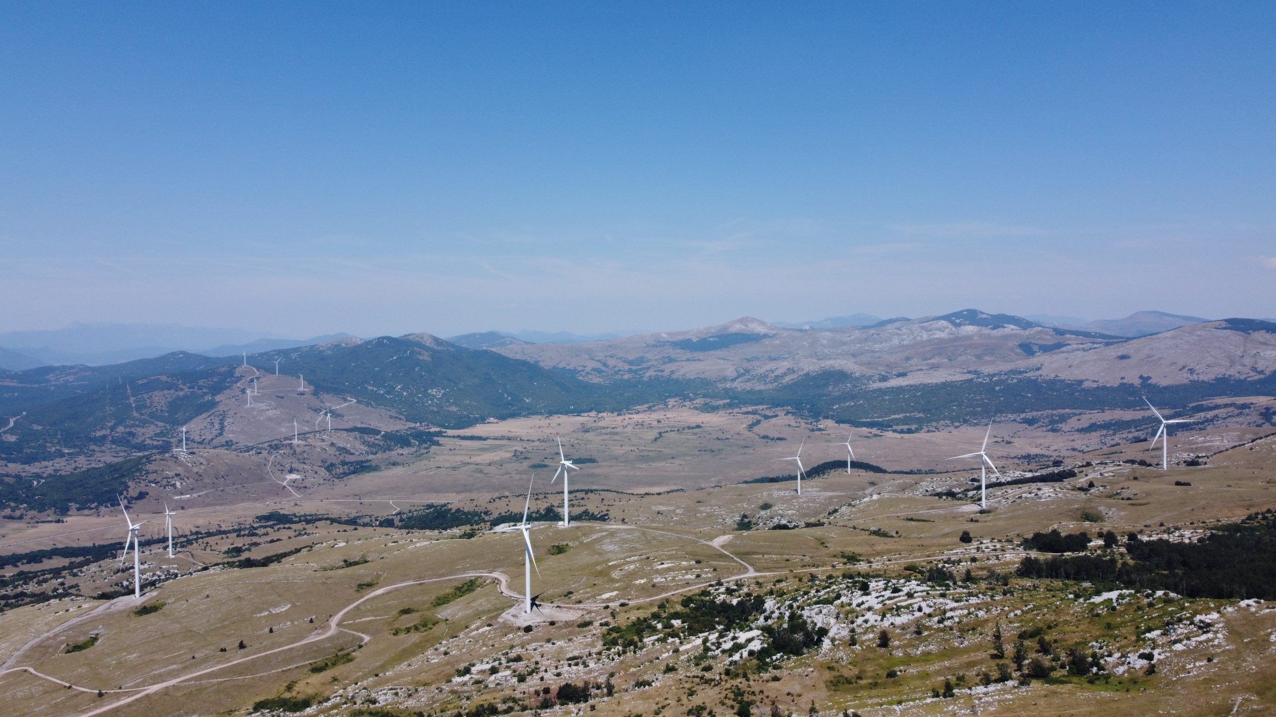
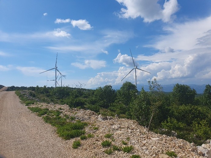
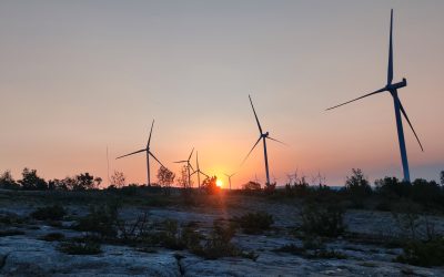
At the same time, wind farms are built in open landscapes—ridges, plains, coastal zones—precisely because these areas offer strong and consistent wind. These landscapes are also used by birds for flight, foraging, migration, and dispersal. As a result, wind energy and bird ecology sometimes intersect in physical space.

This intersection does not automatically imply a problem.

Most birds avoid turbines successfully, and many wind farms operate with minimal or negligible impacts on bird populations. However, for certain species, under specific conditions, wind turbines can pose a collision risk. Whether that risk is relevant or insignificant cannot be assumed—it needs to be quantified.

This is where Collision Risk Analysis (CRA) comes in.

Collision Risk Analysis is a pre-construction assessment used to estimate how often birds may collide with turbine blades once a wind farm is operational. Its purpose is not to argue for or against wind energy, but to provide an evidence-based evaluation that allows developers, regulators, and conservation authorities to make informed decisions.

CRA is carried out before construction, when turbine layouts can still be adjusted, mitigation measures planned, and uncertainties addressed. It translates field observations of bird flight behaviour into a predictive framework that estimates collision risk under realistic operating conditions.

Importantly, CRA acknowledges two key facts at the same time:

• Wind farms are an essential component of sustainable energy systems.

• Wildlife impacts, where they exist, should be identified, assessed, and managed responsibly.

Rather than relying on assumptions or general statements, CRA provides a standardized way to answer a practical question:

How often are birds expected to enter the rotor-swept area of turbines, and what is the likelihood that this results in a collision?

To answer that, CRA combines ecological data (such as bird flight activity and height) with technical information about turbines (such as rotor size and rotation speed). The result is a quantitative estimate of collision risk, usually expressed on a monthly and annual basis for individual species.

This approach allows potential impacts to be:

• compared between species,

• evaluated across seasons,

• and placed into a broader ecological and regulatory context.

Once the rationale for Collision Risk Analysis is clear, the methodology itself becomes much easier to understand. What follows is not a checklist, but a structured way of thinking about how birds move through space—and how wind turbines operate within that same space.

The Practical Guide: How to Do Collision Risk Analysis Step by Step (Pre-Construction)

You’ve got the “why.” Now you want the “how.”

Here’s the good news: pre-construction collision risk analysis is not magic. It’s a repeatable process that turns field observations into a quantitative estimate of risk.

Here’s the other good news: you don’t need a PhD to follow it. You just need to be disciplined about units, and consistent about what each number represents.

Think of CRA like cooking: if you measure ingredients correctly, the recipe works. If you eyeball the salt, you might ruin dinner.

Let’s walk through it.

Step 0: Define your turbine geometry (because it controls “the danger zone”)

Before you touch bird data, define the rotor-swept height band. This is the vertical slice of air where collisions can happen.

You need:

• Hub height (H) = height of the rotor center above ground

• Rotor radius (R) = half the rotor diameter

The rotor-swept band is:

Lower tip height = H − R
Upper tip height = H + R

Everything else in the analysis depends on this, because birds flying outside that band cannot collide with blades.

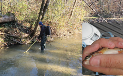
Step 1: Collect flight activity data (Vantage Point surveys)

The basic idea of a vantage point (VP) survey is simple:

• you sit at a fixed location,

• you scan a defined area (of construction site),

• and you record every relevant flight you observe.

But CRA requires one specific type of VP output:

time spent flying (not just “number of birds”).

That’s why CRA loves bird-seconds:

• one bird flying for 60 seconds = 60 bird-seconds

• three birds flying for 20 seconds each = also 60 bird-seconds

This is the best way to capture “how much airspace use” is happening.

For each observation you typically need:

• species

• flight duration (seconds)

• flight height band (or estimate)

• where it occurred (inside your study area)

• which VP recorded it

• time spent observing (effort)

Step 2: Decide how you’ll treat multiple VPs (this matters a lot)

Take time to plan how to set up Vantage Points during the planning phase, and your life will be easier during analysis!

If you have more than one VP, you have two common situations:

1. VPs observed simultaneously
   You need to avoid double-counting the same flight.

2. VPs observed at different times (not simultaneous)
   This is simpler: you can combine them as independent samples of the same site.

In pre-construction work, the second case is very common. In that case, you typically produce one final monthly dataset by aggregating across VPs.

The key principle: combine VPs in a way that respects effort (how long you watched) and the area you covered (how much space you could see). YOu also need to be aware if any of the VPs view areas overlap, for the calculation of visibility area.

Step 3: Calculate DA (bird density in the air)

This is where CRA becomes “a model” and not just “a survey summary.”

The Band approach wants a measure called:

DA_birds_km² = average instantaneous density of flying birds (birds per km²), at any height.

Here’s the cleanest way to compute it from VP data:

DA = total bird-seconds / (observation seconds × visible area in km²)

*there are other ways of calculating DA, but I am just talking how we do it in BIOTA.

Let’s translate that:

• total bird-seconds = sum of all flight durations for that species in that month

• observation seconds = total time you spent watching during that month

• visible area (km²) = the area of airspace you were effectively sampling from VPs

This produces something intuitive:

“At a random moment, how many birds of this species are typically in the sky above one square kilometre?”

If you only remember one “don’t mess this up” rule, it’s this:

***DA divides by area.
It does not multiply by area.

Step 4: Calculate Q2R (the fraction of activity inside rotor height)

DA tells you “birds are in the air.”
Q2R tells you “how much of that air use is inside the rotor height.”

Q2R is simply the proportion of your recorded flight time that falls inside the rotor band:

Q2R = bird-seconds inside (H−R to H+R) / total bird-seconds (all heights)

If your VP data is stored by height bands, this is easy:

• sum the time in bins that fall inside rotor heights

• divide by total time across all height bins

If a height band overlaps the rotor boundary, you can approximate by splitting proportionally by bin width. For most pre-construction assessments, a reasonable approximation is acceptable as long as you document it.

Step 6: Decide if night activity matters (for most raptors, it doesn’t)

CRA often works in monthly time steps, and the model needs to know how many “active seconds” exist in the month.

For many species, night flight is real (migrants, seabirds, etc.).
For most diurnal raptors, it’s effectively zero.

In practice, you create:

Active hours = daylight hours + (night hours × nocturnal fraction)

Nocturnal fraction might be:

• 0.0 for strictly diurnal

• 0.25 for slight crepuscular

• higher for truly nocturnal or nocturnal migrants

If you have a nocturnal rank table, you just map it to a fraction and apply it consistently.

Step 7: Calculate “transits” through the rotor disc (how often birds pass through)

Now we’re ready for the first big modeled output.

A “transit” is one bird passing through the rotor-swept airspace once.

The Band basic model estimates transits using:

• bird density in the air (DA)

• rotor area

• flight speed

• proportion at rotor height (Q2R)

• active time

• number of turbines

• operational fraction (if included)

If you’ve set up DA and Q2R correctly, the transit calculation becomes straightforward.

This step answers:

“How many opportunities for collision exist, before considering blade rotation and avoidance?”

Step 8: Compute single-transit collision probability (the “one pass” risk)

This is the part called “Stage C” in many templates.

Here you estimate:

“If a bird passes through the rotor disc once, what is the chance it gets hit?”

This depends on turbine mechanics and bird size:

• rotor speed (rpm)

• blade width profile (chord)

• number of blades

• pitch / blade angle

• bird length and wingspan

• relative wind direction (upwind vs downwind)

And here’s a practical reality of pre-construction work:

You often don’t have perfect blade profile data.

When that happens, you use:

• a standard generic blade profile for the turbine class,

• a reasonable rpm range,

• and document assumptions clearly.

If your spreadsheet shows blanks in Stage C, the culprit is usually:

• missing blade profile values,

• broken references,

• or macros disabled.

Step 9: Apply avoidance (because birds aren’t dumb)

If you stop at “collision probability,” you’ll overestimate impacts.

Avoidance rate reflects that birds typically detect and avoid turbines.

Final collision estimate:

Collisions = (Transits × single-transit probability) × (1 − avoidance rate)

Avoidance is often the biggest uncertainty, so best practice is to:

• use standard defaults (by species group)

• and/or run sensitivity cases (e.g., 0.95, 0.98, 0.99)

This makes your report more honest and more defensible.

Step 10: Summarize results the way authorities expect

Decision-makers (Ministry, Agencies) want results that are:

• species-specific

• monthly (seasonal pattern)

• annual totals

• transparent assumptions

A typical output includes:

• a table of monthly transits / collisions (before & after avoidance)

• annual totals

• a short explanation of assumptions

• a clear statement of uncertainty (especially blade profile and operational time)

This is our recipe — a practical, transparent way to turn bird flight data into a defensible collision risk assessment before a wind farm is built. We use it in different types of Nature Impact Assessements for wind and solar developers.
If you follow these steps, you’re now equipped to carry out a Collision Risk Analysis that regulators can understand and projects can stand behind.
And if you do it differently, improve a step, or challenge an assumption — even better.
That’s how good methods evolve, and we’re always happy to hear about it.