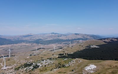
Let me tell you about a job that sounds like a setup for a weird indie horror film: waking up at sunrise, heading out to a remote wind farm, and walking in careful circles under 100-meter turbines looking for dead bats.

No, really — this is a real thing. It’s called post-construction monitoring, and it’s one of those unsung scientific rituals that lives quietly behind the glossy sustainability reports and wind energy press releases. Because while wind energy is a massive step toward a greener planet, it also comes with its own shadow: wildlife collisions, especially bats.

Now, here’s the thing most people miss. You’d think it’s just a matter of counting dead animals and calling it a day. Like some grim Easter egg hunt. But nah. That would be too easy. The reality is we almost never see the full picture. Some bats fall too far from the search zone. Some get snatched up by scavengers before the survey team arrives. Some just go undetected because even trained eyes can miss something the size of a fig bar blending into rocks and brush.

So when a surveyor finds, say, five bat carcasses under a turbine, we all know it’s not really five. The question is — how many did actually die?

And that’s where it gets fun. Because now we’ve entered the world of probability, modeling, and ecological CSI. We’re not just asking, “what happened?” We’re trying to infer what actually happened from the bits and pieces left behind.

This is where advanced statistical tools like Fatality Estimator and GenEst come in. These both tools were developed by researchers at the U.S. Geological Survey (USGS), in collaboration with statisticians, ecologists, and industry partners, as part of a broader effort to create standardized, science-based methods for estimating wildlife mortality at wind energy facilities.

Now, I’ll be honest — these tools don’t sound sexy. They sound like spreadsheets with better fonts. But they’re kind of brilliant. They take your messy, partial, biased field data and run it through algorithms that account for things like searcher efficiency (how likely a human is to find a dead bat if it’s there), carcass persistence (how long a carcass sticks around before it’s eaten or decomposes), and how often and how thoroughly the area was searched. These tools are basically probability machines with a knack for wildlife forensics.

“In God We Trust, All Others Bring Data”

Before the data crunching begins, there’s the grind of fieldwork — and it’s surprisingly methodical. Every post-construction monitoring campaign kicks off with a calibration phase, because no one wants to base a statistical model on wishful thinking. So here’s how it goes: before the actual survey starts, the biologists — often bat experts themselves — head out and plant small carcasses, usually mice, across the site. Why mice? They’re close enough in size and squishiness to mimic a fallen bat, and they’re readily available. One researcher hides them, carefully noting the location, and then another comes through pretending not to know where anything is, scanning the terrain like a real survey would. This is how we measure Searcher Efficiency — how good a person actually is at spotting carcasses in real-world conditions, with all the wind, sun glare, grass height, and distractions baked in. At the same time, some of those test carcasses are left out for days or even weeks, checked regularly to see how long they remain before scavengers, ants, rain, or time itself makes them disappear. That’s Carcass Persistence, and it tells us how likely it is that something died without a trace. Only after all this calibration do the real surveys begin, methodically walking turbine pads, eyes scanning, data forms in hand, ready to record actual casualties. And get this — in some places, they do the whole thing with specially trained dogs. These canines are amazing at sniffing out carcasses, but just like humans, they need calibration too, with their own searcher efficiency scores built into the model.

Fatality Estimator is the original — kind of the OG in this space. It’s simple, accessible, and does the job well. But GenEst? That’s the Tesla of mortality estimation. Built in R (which basically means it’s a tool for people who think Excel is too cute), GenEst can handle wild variability: irregular search schedules, different turbines, seasonal shifts, the whole shebang. It doesn’t just spit out a number. It gives you uncertainty. Confidence intervals. Ranges you can defend in a report to a government regulator who’s got their skeptical eyebrows locked and loaded.

Now, when you plug your field data into GenEst, you don’t get a magic number — you get a spectrum of truth. Maybe it says, “Hey, we found 5 bats, but given everything we know about this site — scavenger rates, search coverage, detection probability — the real number’s probably somewhere between 12 and 18.” That, my friend, is a very grounded way of facing ecological reality.

What’s wild is that we need these tools not just for science, but for permits. For environmental ethics. For the soul of what green energy even means. Because you can’t call wind energy clean if it’s quietly scrubbing out species behind the scenes. You can’t fight climate change and forget the tiny mammals who eat their weight in mosquitoes every night.

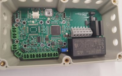
The cool part? This space is getting smarter every year. We’re starting to see tech emerge that lets turbines respond in real-time to bat activity. Cameras. Acoustic detectors. Machine learning models trained to shut down turbines at dusk during migration peaks. Imagine a wind turbine that knows when to chill out to save a life. That’s where we’re going.

So yeah. Maybe post-construction monitoring sounds niche, maybe even a little weird. But it’s also this beautiful, complex ballet of ecology, math, and technology. It’s about making energy better — not just cleaner, but kinder. And the people doing it? They’re out there before sunrise, measuring what most of us never see, using tools most of us don’t understand, making decisions that echo louder than the turbine blades above their heads.

In a world obsessed with scale, it’s nice to know someone’s still counting the small things.

Even bats. Especially bats.

Practical guide: how we actually calculated Wind Farm Fatalities (bats or birds)

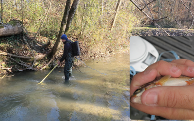
So, you’ve tromped through the wind farm, sunburnt and smelling like sweat and crushed sagebrush. You’ve got a clipboard full of carcass locations, trial mice, and days of search effort under your belt. Now what?

Now comes the real magic: turning your field notes into hard numbers — and that’s where the Fatality Estimator and GenEst tools come in. These are not just some dusty spreadsheets; they’re statistically robust, government-backed, field-tested software packages that help you go from “we found 3 bats” to “we estimate 48.6 bats were killed this season, with a 95% confidence interval.” Sounds fancy — and it is.

But first, let’s go back to the start…

Setting Up the Fieldwork – You Can’t Model What You Don’t Measure

Before you even think about loading data into a computer, you need to run what’s basically a statistical calibration exercise disguised as fieldwork. This is where bat biologists get creative.

They take small carcasses — often mice, which are close enough in body mass and visual detectability to bats — and scatter them around the turbines like biological easter eggs. Another person then walks the site pretending it’s a real survey, without knowing where the “planted” bodies are. This gives you the Searcher Efficiency: the percentage of carcasses a human (or dog!) can actually detect under field conditions.

Some carcasses are left in the field over time, with checks every few days. This tells you how long they stick around before scavengers, weather, or rot make them vanish — aka Carcass Persistence.

Without these two calibrations, your actual survey data is mostly vibes and guesswork. But with them? You can start telling a story with real statistical teeth.

Using the Fatality Estimator: Old-School, Reliable

Let’s start with the OG tool — the Fatality Estimator. It’s a standalone Windows program developed by the USGS. It’s a little clunky, but like a good 4×4, it’ll get you there if you treat it right.

Here’s how the workflow looks:

• Prepare your data in .CSV files with strict formatting rules: comma-delimited, no stray characters, and dates in MM/DD/YYYY format. Any wrong semicolon or non-English letter in a file path? Boom — it crashes.

• You need three input tables:

  • Fatality data: each carcass found, when, where, what species.

  • SE trial data: when you planted your test mice and whether they were found.

  • CP trial data: how long each carcass lasted in the field.

• Start by doing a test run with 1 bootstrap to check if everything loads. If it runs, you’re golden.

• Then launch the real analysis with 5,000 bootstraps. This gives you robust confidence intervals on mortality estimates.

It’s picky. If your “visibility” covariate only has one level, or your dates are out of order, or your turbine names aren’t exactly the same in every table — the software will throw a tantrum. But once you get past the tantrums? You’ve got mortality estimates you can put in a peer-reviewed paper.

📝 Pro Tip: If you found fewer than 5 carcasses, the tool recommends switching to the Evidence of Absence software (EoA) — but you can also just… go back and search a bit more if that’s logistically possible. Trust me, it’s easier than EoA.

Enter GenEst – The R-Powered Upgrade

GenEst is the younger, smarter sibling of the Fatality Estimator — built in R and backed by the USGS again. It’s shinier, more flexible, and comes with a Shiny App GUI that makes your browser feel like mission control.

Step-by-step, this is how you do it:

1. Install R & RStudio (if you haven’t already).

2. Run: install.packages("GenEst", dependencies = TRUE)

3. Organize your project folder: everything goes in .csv, decimal separator must be . and not ,.

4. Launch GenEst: GenEst() or runGenEst() from the R console.

5. Upload these 4 key files in the app:

   • CO (Carcass Observations) – when/where bats were found.

   • SE (Searcher Efficiency) – your test mouse data.

   • CP (Carcass Persistence) – how long they lasted.

   • SS (Search Schedule) – what turbine was searched on what date.

Now you step through the interface, left to right:

• SE tab: Select the right columns (s1, s2, s3…), run the model, and download the output.

• CP tab: Choose date columns, run survival models (Weibull is a good start), download again.

• Mortality Estimation: Select your SE/CP models, enter how many turbines were surveyed vs. total, and hit “Estimate”.

Each time, GenEst gives you beautiful plots, detection probabilities, and — most importantly — estimated fatalities with confidence intervals.

You can even go wild and break it down by species, turbine, season, or visibility class. Want to know which turbine is your bat-killer hotspot? GenEst will tell you.

Final Tips Before You Rage-Quit

• Keep your turbine names identical across all files (t12 ≠ T12 ≠ t012).

• Make sure dates are in U.S. format (MM/DD/YYYY) and in order.

• Don’t use semicolons or funny characters — this thing hates Croatian encoding quirks like č, ć, š, ž, or đ in folder names.

• Always test with 1 bootstrap before running 5,000. Saves you headaches.

From Field Boots to Confidence Intervals

These tools — Fatality Estimator and GenEst — are the real deal. They’re not just statistical busywork; they let you tell a defensible story about wildlife mortality in the age of renewable energy. It’s where field biology, ecology, and data science collide.

And the best part? Once you’ve done it a few times, it starts to feel like magic. You go from “here’s a list of carcasses” to “here’s the real-world impact of our infrastructure — with math to back it up.” I just hate that R requires razor precision and any wrong dot (.) can couse a crash and you have to redo the analysis. So check your input files 10 times before running.

Now go try it out!