Since 2012, the monitoring of the olm population has been carried out as part of the conservation project PROTEUS aimed at protecting this enigmatic species in South East Europe. Population monitoring is essential for conservation authorities to estimate the number of individuals of protected species at targeted sites, allowing them to plan appropriate conservation activities. BIOTA, a specialized organization, has developed a methodology for assessing both absolute and relative population sizes of endangered species. To monitor the elusive olm, we created a method that combines cave diving (speleodiving) with population assessment using line transects. This scientifically grounded procedure enables accurate and repeatable estimates of the olm’s absolute population size, allowing for comparisons between different locations or for long-term monitoring at the same site.

Cave Diving

When people talk about speleodiving, they often imagine diving in terrestrial cave systems, including springs, sinkholes, pits, and caves. This type of diving takes place in freshwater, which is generally much colder than seawater, with average temperatures ranging between 8 and 12 °C.

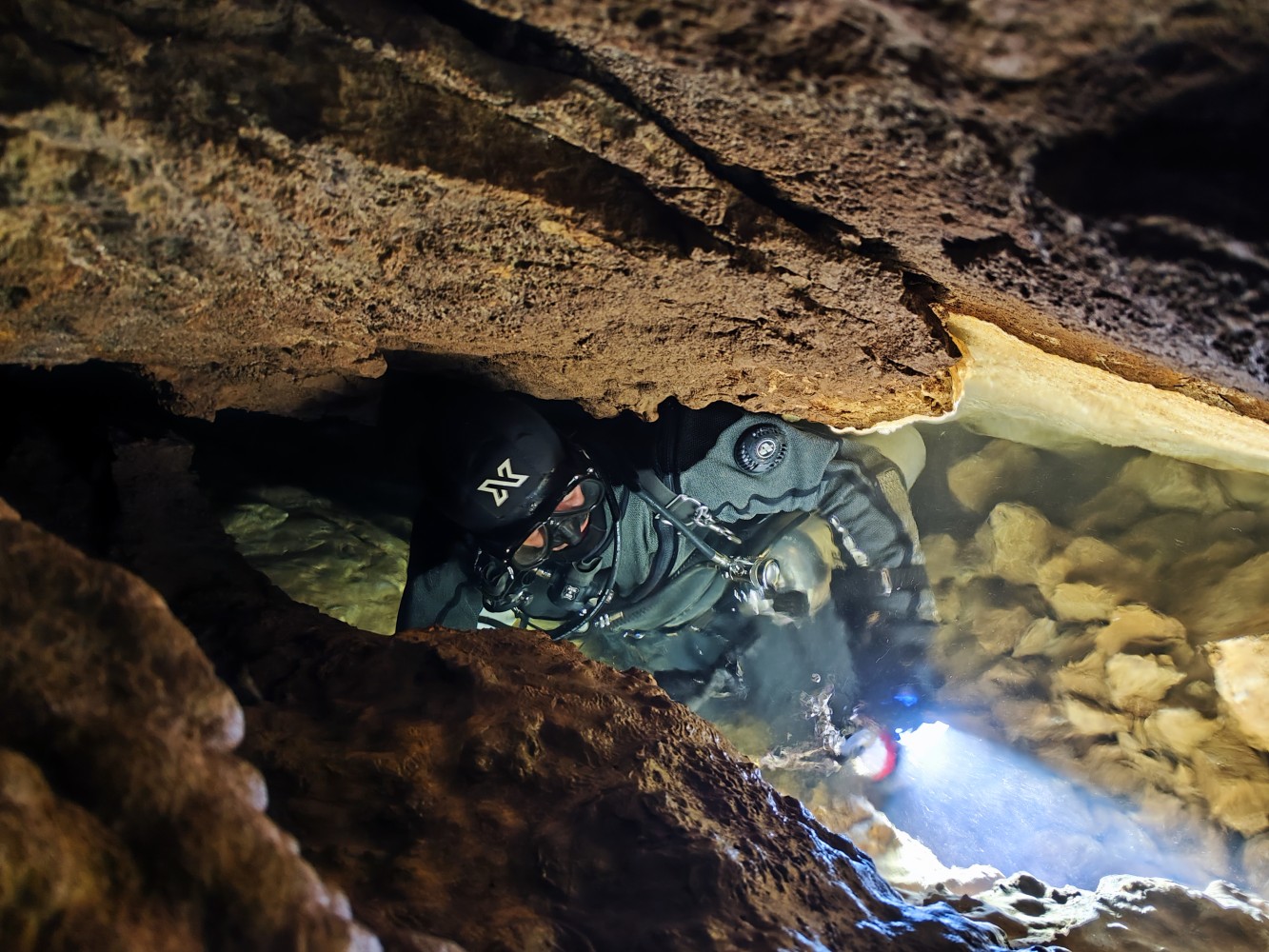
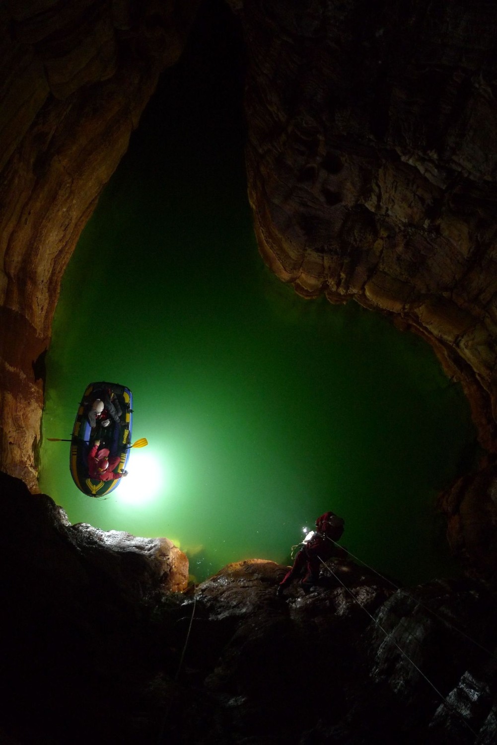
For example, diving in Jablanova Cave near Nikšić, Montenegro, was conducted as part of BIOTA’s research into cave fauna in the Nikšić field. Diving in such environments requires knowledge of speleology, as siphons (water-filled passages) are typically found at the ends of channels and cave systems, requiring caving techniques to access. Croatia is rich in stunning, deep springs and numerous caves, many of which remain unexplored. Cave siphon diving is often the next step after cavers encounter a water barrier (a siphon). Diving in deeper cave siphons is considered the most complex form of speleodiving, requiring a large, well-coordinated team to transport equipment, while divers themselves must be experienced speleologists able to navigate deep passages using ropes.

Population Estimation

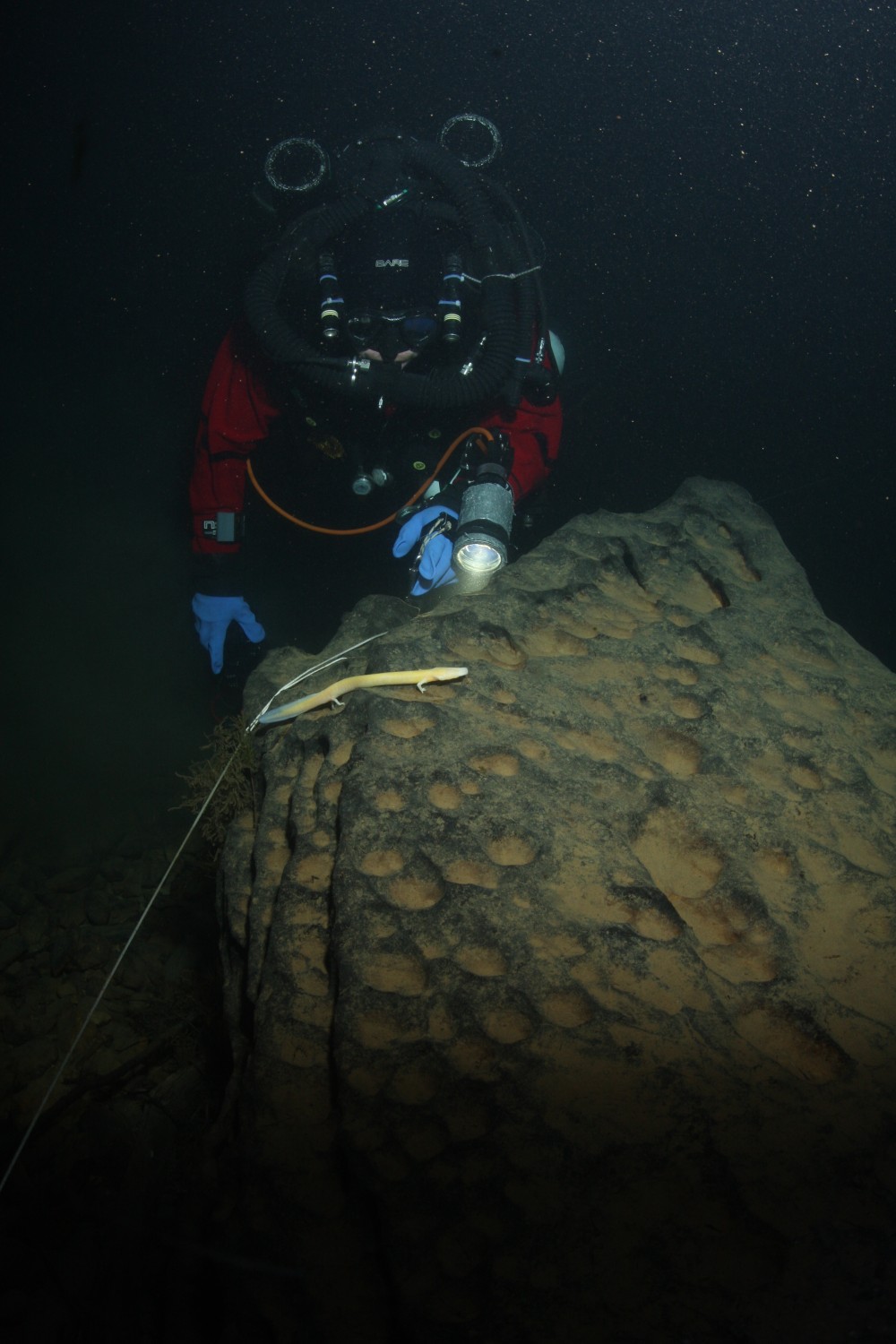
Monitoring of the olm population is conducted using line transect methodology during cave dives. A researcher, who is also a cave diver, follows a pre-defined transect line (a line set up in advance, also serving as a safety line for emergencies) of a known length. The diver records all individuals seen in front, to the left, and to the right, noting their distance from the transect line. This distance is measured as a perpendicular line from the individual to the transect line, and the measurements are recorded with an accuracy of 0.1 meters in the diver’s logbook.

It is critical for the divers to swim slowly along the transect line to observe as many individuals as possible. However, they must not move too slowly, as this could disturb the monitoring process (animals ahead of the diver may flee before being recorded, and previously recorded individuals could be counted twice). If an olm is directly on the transect line, its distance is recorded as 0 meters from the line.

For safety and protocol, two researchers are involved in the monitoring process. The first researcher counts the individuals, while the second monitors environmental parameters and ensures safety. It is important to note that the goal is not necessarily to count as many individuals as possible but to accurately record their perpendicular distance from the transect line. Monitoring is carried out when conditions are ideal, meaning during periods of average or low water flow and when visibility is optimal. Monitoring is not recommended after periods of rain or during high water levels. Ideally, the same two observers should conduct the monitoring year after year. If this is not possible, consistency should at least be maintained throughout a single year’s cycle.

Analysis and Population Size Estimation

The data collected is analyzed to produce an absolute population estimate, calculating the number of olms per square meter and hectare of habitat. These values are then scaled up to the total size of the location (multiplying the number per square meter by the known area of the cave system). The final result is an estimate of the relative population size of mature, sexually mature individuals for the entire location (the known part of the system). This method is sufficient for long-term population trend monitoring.

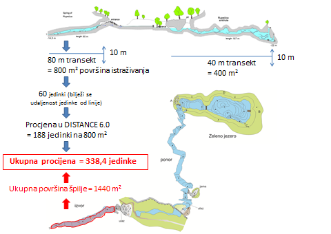
The data is analyzed using the linear transect methodology and the DISTANCE software (version 8.0). This approach is based on data showing how many individuals were observed at a given perpendicular distance and how many went undetected. The distribution and number of detected individuals are used to estimate the number of undetected individuals. By adding these two values, an overall absolute population size can be determined. The DISTANCE software can be downloaded from their website.

For the development of similar species population estimation procedures tailored to your needs, feel free to contact us.