Practical guide: how we actually calculated CPUE (Catch Per Unit Effort)
1. Defining the problem correctly
Before any method was selected, the problem was reframed.
We explicitly accepted that:
-
absolute population size estimation was unlikely to be achievable
-
detection probability was extremely low and variable
-
zero detections could not be interpreted as absence
-
standard outputs (N, density, occupancy probability per grid) were unrealistic goals
The primary objective therefore became:
To establish a repeatable, effort-standardized system that allows comparison through time and space, even when detections are rare.
This single decision guided everything that followed.
2. Field effort standardization (the non-negotiable foundation)
Relative abundance metrics are meaningless without strict effort control.
For every field activity, we recorded:
-
number of observers
-
active survey time (in hours)
-
distance covered (in kilometers)
-
survey type (active search, road transect, incidental)
-
weather conditions and time of day
Only surveys that met predefined comparability criteria were included in calculations (similar season, similar time window, similar survey intent).
This allowed us to later express detections per unit of effort, not as raw counts.
3. Survey types used (and how they were treated analytically)
We did not exclude methods that performed poorly in isolation.
Instead, we treated each method as a filter with its own bias, then decided which outputs were usable.
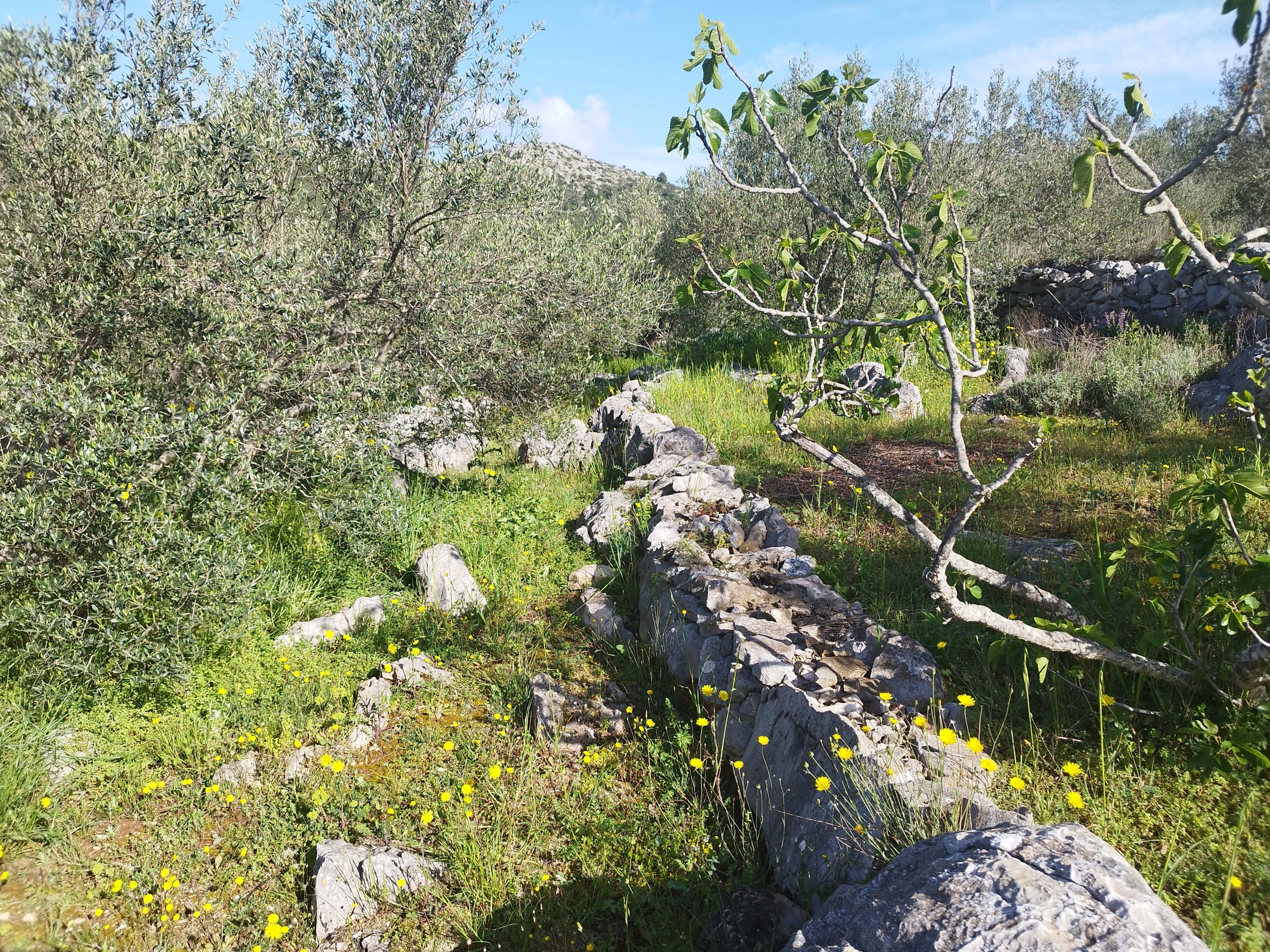
a) Active visual search (time-based)
This included:
-
slow searches of stone walls, rocky slopes, and vegetation
-
targeted microhabitat inspection
-
surveys conducted during biologically plausible activity windows
Output used:
Even when detections were rare, time-based standardization allowed comparison between years.
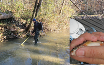
b) Line transects (distance-based)
Transects were walked repeatedly in the same areas.
Outcome:
Decision:
-
transects were not abandoned
-
but their outputs were not used as standalone indicators for the target species
-
they remained useful for other snake species, which later became reference indicators
c) Permanent plots and occupancy framework
Permanent plots were surveyed repeatedly.
Outcome:
Decision:
This is an important point:
Rejecting a method analytically is not the same as abandoning it operationally.
d) Road transects (distance-based, movement-driven)
Road surveys were conducted systematically:
Key insight:
Roads intersect movement, not habitat. For elusive species, this matters more than idealized sampling design.
Output used:
This became one of the most robust indicators for the target species.
4. The core metrics we calculated
We ultimately focused on two primary metrics, both intentionally simple:
Metric 1: Detections per person-hour
RAtime=Total observer hoursNumber of detected individuals
Metric 2: Detections per kilometer
RAdistance=Total kilometers surveyedNumber of detected individuals
These metrics were calculated:
They were never mixed or pooled without clear justification.
5. Why we explicitly avoided “population estimates”
At no point did we extrapolate these metrics to population size.
We did not:
Why?
Because doing so would create false precision.
Relative abundance was treated exactly as that — a relative index, not a hidden proxy for population size.
6. Establishing a baseline (the most important output)
The first years of data were treated as baseline calibration, not evaluation.
Instead of asking:
“Is the population increasing or decreasing?”
We asked:
“What does ‘normal detectability’ look like for this species under standardized effort?”
This baseline now functions as:
-
a reference point for future monitoring
-
a conservation target framework
-
a threshold system for detecting change
7. Adding a third dimension: other snake species as context
Because Zamenis situla produces weak signals on its own, we incorporated other snake species into the analytical framework.
For each year, we calculated the same relative metrics for:
These species were not treated as controls, but as contextual indicators.
Interpretation followed a simple logic:
-
parallel declines → system-level signal
-
divergence → species-specific dynamics
-
stability in common species + change in target species → real biological signal
This step dramatically improved interpretability.
8. What this framework can and cannot do
It can:
-
detect long-term trends
-
provide objective, repeatable indicators
-
support conservation objectives
-
function under extreme detectability constraints
It cannot:
And that is precisely why it works.
9. Why this approach is transferable
This framework is applicable to:
The key is not the species.
The key is the willingness to design monitoring around reality instead of expectation.
Final note for practitioners
If you take only one thing from this guide, let it be this:
When detection is the limiting factor, trend detection beats population estimation.
Once you accept that, monitoring rare and elusive species stops being an exercise in frustration and starts becoming a disciplined, honest form of ecological listening.
And sometimes, that is exactly what conservation needs.


0 Comments